

Abstract
Health managers routinely decide under uncertainty about demand, service times, epidemics and equipment failure. This chapter introduces optimisation under uncertainty (OUU) for health management readers, moving from core concepts and terminology to seven families of methods: scenario analysis, stochastic programming, robust optimisation, distributionally robust optimisation (DRO), chance-constrained programming, fuzzy multi-criteria decision making and simulation-based optimisation. It explains how the type of uncertainty, aleatory or epistemic, guides the choice of method, why expected values alone are insufficient where patient safety is at stake, and why tail-risk measures such as conditional value-at-risk (CVaR) matter in decisions such as blood bank inventory. Advanced approaches, including multi-objective and metamodel-based optimisation, Monte Carlo sampling and machine learning, are outlined, published health care applications are reviewed, and nine worked problems translate the methods into hospital decisions such as operating room scheduling. The chapter closes with the challenges of explainability, computational complexity and clinical applicability.
1. Where Uncertainty Meets Optimisation
Health care is a sector intertwined with uncertainty by its very nature. How many patients an emergency department will admit tomorrow, how long operations will run, how fast an epidemic will spread or when a medical device will fail cannot be known with certainty in advance. Health managers therefore have to decide with incomplete rather than complete information (Heizer et al., 2020). In operations management, optimisation under uncertainty (OUU) provides methods for systematically seeking the best decision even when outcomes cannot be guaranteed (Birge & Louveaux, 2011).
Optimisation is the process of improving (minimising or maximising) an objective function subject to constraints. Uncertainty describes a situation in which the decision maker does not know the true values of some model parameters (Shapiro et al., 2021). Put together, the core question is: how can we make the best decision when some inputs to our model are not certain?
An everyday analogy helps. Suppose a hospital manager is hosting a dinner for 20 people but does not know exactly how many will come. The deterministic approach cooks for exactly 20: if 25 come, there is not enough food; if 12 come, food is wasted. The stochastic approach estimates the probability distribution of attendance from past data and cooks accordingly. The robust approach says that anywhere between 15 and 25 people may come and prepares enough that everyone eats even in the worst case. Translated to the hospital, the food stands for hospital resources, the guests for patient demand, running out of food for being unable to admit patients, and wasted food for idle resources and unnecessary cost.
1.1 Sources of Uncertainty
In operations and health management, uncertainty has three main sources (Mishra et al., 2020; Köbis & Tammer, 2023). Stochastic variability (aleatory uncertainty) is the natural random variation of demand, patient arrival times or surgery durations. It is intrinsic to the system, cannot be removed even by collecting more data, and is modelled with probability distributions. Lack of knowledge (epistemic uncertainty) covers unknown parameters such as the true spread rate of a disease or the effectiveness of a new treatment; it can be reduced over time through research and data collection. Model uncertainty concerns how well the mathematical model represents reality. In health systems all three can be present at once.

Figure 1. Sources of uncertainty in health management.
Uncertainty specific to health care can be grouped more concretely into four types. The first is demand uncertainty: how many patients will arrive at the emergency department and which diseases will cluster cannot be known in advance. The second is duration uncertainty: surgery, treatment and length-of-stay times vary greatly from patient to patient. Wan et al. (2023), studying ICU bed allocation, handled uncertainty in the number of emergency patients and in lengths of stay with a two-stage model and showed that these uncertainties directly affect capacity. The third is resource uncertainty: staff absence, supply disruptions and unexpected equipment failures can interrupt service delivery. The fourth is environmental uncertainty: natural disasters, epidemics and policy changes can transform health systems entirely.
1.2 Why Deterministic Solutions Are Not Enough
Classical (deterministic) optimisation models assume that all parameters are known with certainty, an assumption rarely valid in health care. Denton et al. (2010) showed that deterministic operating room scheduling models that ignore uncertain surgery durations systematically underestimate overtime costs. Bertsimas and Sim (2004) demonstrated that deterministic solutions deteriorate quickly when parameters vary, whereas robust approaches yield far more resilient solutions at very little extra cost. In health management, Saghafian et al. (2015) showed that approaches ignoring uncertainty in emergency department patient flow considerably increase patient waiting times. Masic (2022), examining medical decision making, highlighted two factors that shape decisions: the degree of uncertainty about future events and the utility of the outcomes obtained in each state.
1.3 Historical Development
A Web of Science search for “optimization under uncertainty” identified 246 articles (1990–2026). Their distribution over time shows that the field is growing rapidly: only 10 articles were published in 1990–1999, rising to 114 in 2020–2026. Among the most frequently used approaches are robust optimisation (31 articles), uncertainty quantification (19) and stochastic programming (10). The most cited work is the foundational paper by Rockafellar and Wets (1991), with 867 citations. In PubMed, the query “optimization under uncertainty healthcare” returns 238 results, most published after 2020.

Figure 2. Publication trend for “optimization under uncertainty” (Web of Science, 1990–2026). The approach breakdown within each bar is as shown in the original report’s figure.
2. Core Concepts and Terminology
2.1 Deterministic Versus Stochastic Models
In a deterministic optimisation model all parameters are known and treated as fixed; in a stochastic model they are represented by probability distributions (Birge & Louveaux, 2011). The deterministic model is like planning a picnic on the assumption that the weather will be sunny every day; the stochastic model takes the 30% chance of rain into account and prepares for both sunny and rainy scenarios.
Table 1. Comparison of deterministic and stochastic models
| Feature | Deterministic | Stochastic | Health management example |
|---|---|---|---|
| Parameter | Certain and fixed | Described by a probability distribution | Patients: 120 vs N(120, 15) |
| Decision environment | Complete information | Under uncertainty | Point forecast vs confidence interval |
| Result | A single optimum | Expected-value optimum | One plan vs an adaptive plan |
| Risk measure | None | VaR, CVaR, variance | Probability of excessive waiting |
2.2 Types of Uncertainty
Aleatory uncertainty is the inherent random variability of nature; it cannot be removed even with more data and is modelled with probability distributions. Epistemic uncertainty arises from insufficient information or data; it can be reduced through research and is modelled with interval values, fuzzy sets or probability boxes (Engau & Sigler, 2020; Köbis & Tammer, 2023). The distinction is critical for choosing a modelling approach: aleatory uncertainty is usually addressed with stochastic programming, epistemic uncertainty with robust optimisation and fuzzy approaches (Balasubramanian & Grossmann, 2003).

Figure 3. Matching modelling approaches to the type of uncertainty.
2.3 Risk and Risk Measures
The expected value (EV) is the probability-weighted average across all scenarios: E[f(x, ξ)] = Σ pₛ · f(x, ξₛ). Value at Risk (VaR) is the largest loss that may be encountered at a given confidence level; it answers questions such as “in the worst 5% of cases, what is the maximum waiting time?”. Conditional Value at Risk (CVaR) is the average loss in the scenarios that exceed the VaR threshold; it is more conservative than VaR and captures tail risk better (Rockafellar & Wets, 1991).
2.4 Basic Mathematical Notation
The general form of optimisation under uncertainty is: min E[f(x, ξ)] subject to g(x, ξ) ≤ 0, x ∈ X, where x denotes the decision variables, ξ (xi) the uncertain parameters, f(x, ξ) the objective function, E[·] the expected value operator and X the feasible decision set. In a health management example, a hospital decides how many doctors to keep on duty in the emergency department (x), while the number of patients who will arrive that day is uncertain (ξ). Too few doctors keep costs low but waiting times soar if demand peaks; too many doctors ease service but raise costs. The model seeks the number of doctors that minimises average total cost under uncertain patient demand.
3. Approaches to Optimisation Under Uncertainty
This section covers six core approaches from simplest to hardest: (1) scenario analysis, (2) stochastic programming, (3) robust optimisation, (4) distributionally robust optimisation, (5) chance-constrained programming and (6) fuzzy multi-criteria decision making. For each, a conceptual explanation, a worked problem and empirical evidence from the PubMed literature are presented together.

Figure 4. Approaches to optimisation under uncertainty ordered by complexity.
3.1 Scenario Analysis
Scenario analysis is the simplest and most intuitive method of deciding under uncertainty. A few possible future scenarios are defined and the performance of the decision variables is evaluated under each (Heizer et al., 2020). Rockafellar and Wets (1991) developed the concept of policy aggregation within the scenario-based approach.
Worked Problem 1: Emergency department staffing. The director of a public hospital’s emergency department must choose among three staffing strategies.
Table 2. Scenario-based cost matrix
| Strategy | Low demand (P = 0.3) | Medium demand (P = 0.5) | High demand (P = 0.2) | EMV |
|---|---|---|---|---|
| A (Minimal) | 80,000 TL | 150,000 TL | 320,000 TL | 163,000 TL |
| B (Moderate) | 120,000 TL | 130,000 TL | 180,000 TL | 137,000 TL |
| C (Comprehensive) | 200,000 TL | 160,000 TL | 140,000 TL | 168,000 TL |
Solution: EMV(A) = (0.3 × 80,000) + (0.5 × 150,000) + (0.2 × 320,000) = 163,000 TL; EMV(B) = 137,000 TL; EMV(C) = 168,000 TL. Strategy B, with the lowest expected cost, should be chosen. A minimax regret analysis gives the same answer: Strategy B’s maximum regret is 40,000 TL, the lowest of all strategies (A: 180,000; C: 120,000). Both criteria support Strategy B. Assumptions: the scenarios are mutually exclusive and exhaustive (total probability 1.0); costs are known with certainty under each scenario; the decision maker is risk neutral (EMV criterion).
Worked Problem 2: Expected value of perfect information (EVPI). Using the data from Problem 1, what is perfect information worth? The best strategy in each scenario is: low → A (80,000), medium → B (130,000), high → C (140,000). EVwPI = (0.3 × 80,000) + (0.5 × 130,000) + (0.2 × 140,000) = 117,000 TL. EVPI = 137,000 − 117,000 = 20,000 TL, the maximum that could be paid for a perfect forecasting system.
3.2 Stochastic Programming
Stochastic programming models uncertain parameters with probability distributions and optimises the expected value (Birge & Louveaux, 2011). Diwekar and Kalagnanam (1997) dramatically reduced the computational burden with Hammersley point sampling.
Two-stage stochastic programming. The general form is min cᵀx + Eξ[Q(x, ξ)], where Q(x, ξ) = min {qᵀy : Wy = h(ξ) − T(ξ)x, y ≥ 0}. The first-stage decision x is made before uncertainty is revealed; the second-stage decision y is the recourse taken afterwards. The essence of the model is: decide now in such a way that the initial cost is not too high and correcting course later, once uncertainty is resolved, is not too expensive. In a hospital, the number of nurses rostered for tomorrow is decided today (first stage); if tomorrow brings more patients than expected, extra nurses must be called in or overtime used (second-stage recourse cost).
Worked Problem 3: Hospital drug stock planning (two-stage model). A hospital pharmacy must decide how many boxes of an antibiotic to order at the start of the season. Unit cost is 100 TL and unit use value is 200 TL. Each unused box is returned at 30 TL at the end of the season. When demand cannot be met, an emergency order from an external supplier costs 250 TL per unit. Demand scenarios: low 200 boxes (P = 0.25), medium 350 (P = 0.50), high 500 (P = 0.25).
Step 1, analysis of candidate order quantities. For each candidate x, profit is Profit(x, d) = min(x, d) × 200 + max(0, x − d) × 30 − x × 100 − max(0, d − x) × 250 + max(0, d − x) × 200.
- x = 200: d = 200 gives 20,000 TL; d = 350 gives 40,000 − 20,000 − 37,500 + 30,000 = 12,500 TL; d = 500 gives 40,000 − 20,000 − 75,000 + 60,000 = 5,000 TL. E[Profit] = 0.25 × 20,000 + 0.50 × 12,500 + 0.25 × 5,000 = 12,500 TL.
- x = 350: d = 200 gives 40,000 + 4,500 − 35,000 = 9,500 TL; d = 350 gives 35,000 TL; d = 500 gives 70,000 − 35,000 − 37,500 + 30,000 = 27,500 TL. E[Profit] = 26,750 TL.
- x = 500: d = 200 gives 40,000 + 9,000 − 50,000 = −1,000 TL; d = 350 gives 70,000 + 4,500 − 50,000 = 24,500 TL; d = 500 gives 50,000 TL. E[Profit] = 24,500 TL.
Table 3. Expected profit of candidate order quantities
| Order (x) | E[Profit] |
|---|---|
| 200 | 12,500 TL |
| 350 | 26,750 TL (optimal) |
| 500 | 24,500 TL |
Step 2, critical ratio check. Because demand is always met through recourse, the understocking cost is Cᵤ = 250 − 100 = 150 TL (the difference between emergency and normal supply) and the overstocking cost is Cₒ = 100 − 30 = 70 TL. CR = 150 / (150 + 70) ≈ 0.682. With discrete scenarios, F(200) = 0.25 < 0.682 ≤ F(350) = 0.75, so x* = 350 boxes, consistent with Step 1. Assumptions: single-period decision; unlimited emergency supply at a fixed 250 TL; demand represented by three discrete scenarios.
Empirical evidence. Arab Momeni et al. (2022) studied operating room scheduling during the COVID-19 pandemic and used a stochastic robust optimisation approach to handle uncertainty in elective and emergency surgery durations, incorporating the new constraints imposed by protective guidelines into a mixed-integer model applied to a cardiovascular department in Iran. Shehadeh and Padman (2023) developed a framework to reduce congestion in the recovery unit using the long and highly variable post-operative lengths of stay of cardiovascular surgery patients: machine learning estimated lengths of stay and their distributions, optimisation models scheduled procedures on a rolling basis, and performance was evaluated by simulation.
3.3 Robust Optimisation
Robust optimisation does not require a probability distribution; it defines an uncertainty set in which parameters may lie and optimises for the worst case (Ben-Tal et al., 2009): minx maxξ∈U f(x, ξ). Bertsimas and Sim (2004) eased the problem of over-conservatism with a robust formulation that has an adjustable level of protection. Where stochastic optimisation says “find the decision that is best on average”, robust optimisation says “find the decision that will not break even in the worst case”.
Worked Problem 4: Pandemic capacity planning (robust approach). A provincial health directorate wants to prepare extra bed capacity for a possible outbreak. Daily extra bed demand d lies in [50, 200] with an unknown distribution. Each extra bed costs 5,000 TL to set up; transferring a patient when beds run out costs 15,000 TL per patient; maintaining an unused bed costs 1,000 TL. Cost function: C(x, d) = 5,000x + 1,000 × max(0, x − d) + 15,000 × max(0, d − x).
The balance point C(x, 200) = C(x, 50) gives x = 190.625. Comparing integers: the worst-case cost is 1,100,000 TL for x = 190, 1,096,000 TL for x = 191 and 1,102,000 TL for x = 192. Optimal decision: x* = 191 beds, with the minimum worst-case cost of 1,096,000 TL. Because transferring a patient (15,000 TL) costs 15 times as much as maintaining an empty bed (1,000 TL), the robust approach recommends a solution close to the upper bound (191 of 200), consistent with the principle of patient safety. Assumptions: the cost function is piecewise linear in d; all unit costs are fixed; x is an integer; the uncertainty set U = [50, 200] is known exactly.
Empirical evidence. Aslani et al. (2021) developed a cardinality-constrained robust optimisation model for tactical capacity planning in an outpatient setting; it produced capacity allocations feasible for all demand realisations allowed by the uncertainty budget, guaranteeing 100% feasibility without reaching full conservatism. Fariman et al. (2024) built a robust model for post-disaster blood supply chains using real data from Iran to identify donation centres, medical facilities and new facility needs. Hoffmans-Holtzer et al. (2024) applied robust optimisation to the pre-treatment preparation workflow of a one-stop palliative radiotherapy clinic and, with a genetic algorithm, obtained schedules that reduced patient preparation time by 37%.
3.4 Distributionally Robust Optimisation (DRO)
DRO is a synthesis of stochastic programming and robust optimisation. When the exact distribution of an uncertain parameter is unknown, it assumes that the true distribution belongs to an ambiguity set of possible distributions and optimises the expected value under the worst of them (Jiang & Guan, 2016): minx maxP∈𝒫 EP[f(x, ξ)]. Stochastic programming says “I know the true distribution”; robust optimisation says “I will not use the distribution at all”; DRO says “I do not know the exact distribution, but I know the set of possible ones, so I optimise the expected value against the worst distribution in that set”.
Worked Problem 5: Vaccine stock planning (DRO approach). A provincial health directorate will order seasonal influenza vaccine. Daily demand is estimated at μ = 400 doses with σ = 80 doses, but the true distribution is unknown. Unit vaccine cost is 50 TL, emergency supply per unmet dose 200 TL, and disposal of each unused dose 40 TL.
Solution: understocking cost Cᵤ = 150 TL, overstocking cost Cₒ = 90 TL, CR = 150 / 240 = 0.625. Using Scarf’s distribution-free newsvendor bound: x*DRO = 400 + (80 / 2) × (√1.667 − √0.6) = 400 + 40 × 0.516 ≈ 421 doses. For comparison, the stochastic programming solution under a normal assumption is x*SP ≈ 425 doses. The DRO solution is slightly lower because, in protecting against the worst distribution, it also balances the risk of overstocking; if the normal assumption is wrong, the DRO solution is the more reliable one.
Evidence. Shehadeh and Padman (2022) noted that the distribution of surgery duration varies greatly between patients. Estimating these distributions with machine learning methods such as quantile regression forests and integrating them into the optimisation model strengthens the distributionally robust approach.
3.5 Chance-Constrained Programming
Chance-constrained programming requires constraints to be satisfied with a specified probability (Wendt et al., 2002): min f(x) subject to P[g(x, ξ) ≤ 0] ≥ 1 − α. A deterministic model says “satisfy the constraint with certainty”, robust optimisation usually says “satisfy it even in the worst case”, and chance-constrained programming says “satisfy it at a given confidence level”. It offers a more balanced solution when full assurance would be too costly.
Worked Problem 6: Emergency department waiting time. Patient waiting time W ~ N(μ, σ²) with μ = 22 minutes and σ = 6 minutes. The manager wants waiting time not to exceed 30 minutes with 95% probability. Solution: Z = (30 − 22) / 6 = 1.33; Φ(1.33) ≈ 0.908, so P(W ≤ 30) ≈ 90.8% < 95% and the target is not met. A 95% guarantee requires Z ≥ 1.645. Either reduce the mean (with σ = 6 fixed, μ ≤ 20.13 minutes) or reduce variability (with μ = 22 fixed, σ ≤ 4.86 minutes).
3.6 Fuzzy Multi-Criteria Decision Making
Fuzzy multi-criteria decision making (FMCDM) represents uncertainty with fuzzy sets and membership functions. It is preferred when parameters can be expressed by expert judgement in linguistic terms such as “approximately”, “low” or “high”. Büyüközkan et al. (2011) presented a fuzzy AHP-based framework for assessing health service quality.
Worked Problem 7: Supplier selection with fuzzy evaluation. A hospital will choose a medical consumables supplier. Three candidates are rated with triangular fuzzy numbers on three criteria: price (w = 0.40), delivery reliability (w = 0.35) and product quality (w = 0.25). Defuzzification uses the centroid of the triangular fuzzy number, (a + b + c) / 3.
Table 4. Supplier evaluation with triangular fuzzy numbers
| Supplier | Price (w = 0.40) | Reliability (w = 0.35) | Quality (w = 0.25) | Score |
|---|---|---|---|---|
| T1 | (6, 7, 8) | (5, 6, 7) | (7, 8, 9) | 6.90 |
| T2 | (7, 8, 9) | (6, 7, 8) | (5, 6, 7) | 7.15 |
| T3 | (8, 9, 10) | (7, 8, 9) | (6, 7, 8) | 8.15 |
T3 has the highest score. Calculation note: the Turkish report lists 7.05 for T2 and 8.10 for T3; with the stated weights and centroids the weighted sums are 0.40 × 8 + 0.35 × 7 + 0.25 × 6 = 7.15 and 0.40 × 9 + 0.35 × 8 + 0.25 × 7 = 8.15. The ranking is unchanged.
3.7 Simulation-Based Optimisation
Simulation-based optimisation is used in complex systems where an analytical solution is not possible. A computer model of the system is built and alternative decisions are simulated thousands of times to identify the best-performing one. Daldoul et al. (2023) combined optimisation and simulation in an emergency department in Tunisia: a stochastic mixed-integer linear programme that accounted for uncertain arrivals and service times first set the optimal numbers of staff and beds, then discrete-event simulation evaluated this allocation under different patient scheduling rules. The approach reduced length of stay by 44.55% on average.
4. Advanced Approaches
4.1 Multi-Objective Optimisation and Pareto Efficiency
Health management decisions usually require balancing several objectives at once. Multi-objective optimisation seeks not a single “best” solution but the Pareto-efficient set, in which no objective can be improved without worsening another. Engau and Sigler (2020) defined Pareto optimality under uncertainty based on six ordering relations. Roshanaei et al. (2017) developed a collaborative operating room planning and scheduling model. In PubMed evidence, Wan et al. (2023) simultaneously minimised the number of required ICU beds, maximised resource utilisation and maximised patient admission; their improved NSGA-II algorithm required 9.8% and 5.1% fewer ICU beds than the MOSA and MOTS algorithms.
4.2 Metamodel-Based Optimisation
Simulating a complex health system for every scenario can be computationally prohibitive. Metamodels represent the input-output relationship of a complex simulation with a simplified statistical model. Jin et al. (2003) compared metamodelling techniques such as Kriging and polynomial regression and found Kriging superior for nonlinear response surfaces. Ng and Willcox (2014) showed that multifidelity approaches combining models of different accuracy can save up to 90% of computation.
4.3 Monte Carlo Simulation and Sampling Techniques
Monte Carlo simulation estimates the statistical distribution of system performance from random samples. Diwekar and Kalagnanam (1997) showed that Hammersley sampling achieves equivalent accuracy with ten times fewer samples than standard Monte Carlo. Guth and Van Barel (2023) proved that multilevel quasi-Monte Carlo converges faster than standard Monte Carlo.
4.4 Artificial Intelligence and Machine Learning in OUU
Ning and You (2019) reviewed the integration of big data and deep learning with OUU and identified three contributions: more accurate estimation of uncertain parameters through deep learning, sequential decision making under uncertainty through reinforcement learning, and scenario generation with generative adversarial networks. Hill et al. (2025) used gradient boosting models to analyse emergency medical service response times and found that weather, call priority and resource constraints drive response-time variability. Such predictive analytics provide a basis for adaptive resource allocation models.
4.5 Maintenance Scheduling and Reliability Optimisation
Vassiliadis and Pistikopoulos (2001) developed a system effectiveness measure and a mixed-integer nonlinear programming model to derive optimal maintenance policies under uncertain parameters. The approach can be adapted directly to the maintenance timing of MRI units, CT scanners and laboratory equipment in hospitals.
4.6 Decision Trees and Probabilistic Decision Graphs
Jensen and Nielsen (2011; 2013) presented a comprehensive framework of probabilistic decision graphs for sequential decision problems under uncertainty. Tolpin and Shimony (2012) extended the value-of-information concept to a semi-myopic framework, systematising the evaluation of the cost of gathering additional information against its benefit. In health management, decision trees are widely used in clinical diagnostic algorithms, treatment protocol selection and cost-effectiveness analysis.
5. Applications in Health Management and Worked Problems
5.1 Worked Problem 8: Operating Room Scheduling
An operating room manager plans three operations for one day. The theatre runs 480 minutes a day; overtime costs 50 TL per minute; the target is no overtime with 90% probability.
Table 5. Surgery duration estimates
| Operation | Mean duration (min) | Standard deviation (min) | Distribution |
|---|---|---|---|
| A (General surgery) | 120 | 20 | Normal |
| B (Orthopaedics) | 150 | 30 | Normal |
| C (Ophthalmology) | 90 | 15 | Normal |
Solution: for independent normal durations the total is also normal: μT = 120 + 150 + 90 = 360 minutes and σT = √(20² + 30² + 15²) = √1525 ≈ 39.05 minutes. Chance constraint: P(T ≤ 480) = Φ((480 − 360) / 39.05) = Φ(3.07) ≈ 0.9989 > 0.90, so the constraint is comfortably met. Expected overtime is E[(T − 480)⁺] = σT × L(z), where L(z) = φ(z) − z[1 − Φ(z)] is the standard normal loss function. With z = 3.07, L(3.07) ≈ 0.00029, so expected overtime ≈ 0.012 minutes and the expected overtime cost is about 0.6 TL per day.
If a fourth operation is added (D: μ = 100, σ = 25): μT = 460 and σT = √2150 ≈ 46.37 minutes. P(T ≤ 480) = Φ(0.43) ≈ 0.667 < 0.90, so the constraint is violated. L(0.43) ≈ 0.220, expected overtime ≈ 10.2 minutes and expected overtime cost ≈ 510 TL per day. Calculation note: the Turkish report uses 0.00106 for L(3.07), which is the tail probability 1 − Φ(3.07) rather than the loss function, giving 0.041 minutes and 2.07 TL; for the four-operation case it reports 10.42 minutes and 521 TL. The conclusion (three operations are safe, a fourth breaks the 90% target) is unaffected. Assumptions: independent durations; normal distribution; changeover times not modelled.
5.2 Worked Problem 9: Blood Bank Inventory (CVaR Approach)
A regional blood centre wants to set the daily order for A Rh-positive blood. Supply cost is 300 TL per unit ordered, disposal cost 100 TL per unused unit and the emergency procurement cost 800 TL per unit short. Four equally likely demand scenarios: 25, 35, 45 and 60 units (P = 0.25 each). Cost function: C(x, d) = 300x + 100 × max(0, x − d) + 800 × max(0, d − x).
Step 1, broad candidate analysis. Order quantities x = 25, 30, 35, 40, 45, 50 and 60 are compared systematically, computing the expected cost (EMV) and CVaR80 for each. With four equally likely scenarios, the worst 20% of outcomes falls entirely within the worst scenario, so CVaR80 equals the highest scenario cost.
Table 6. EMV and CVaR80 of candidate order quantities (TL)
| x | C(x, 25) | C(x, 35) | C(x, 45) | C(x, 60) | EMV | CVaR80 |
|---|---|---|---|---|---|---|
| 25 | 7,500 | 15,500 | 23,500 | 35,500 | 20,500 | 35,500 |
| 30 | 9,500 | 13,000 | 21,000 | 33,000 | 19,125 | 33,000 |
| 35 | 11,500 | 10,500 | 18,500 | 30,500 | 17,750 | 30,500 |
| 40 | 13,500 | 12,500 | 16,000 | 28,000 | 17,500 | 28,000 |
| 45 | 15,500 | 14,500 | 13,500 | 25,500 | 17,250 | 25,500 |
| 50 | 17,500 | 16,500 | 15,500 | 23,000 | 18,125 | 23,000 |
| 60 | 21,500 | 20,500 | 19,500 | 18,000 | 19,875 | 21,500 |
Step 2, critical ratio check. Under this cost function, one more unit ordered costs 300 TL (plus 100 TL disposal if unused) and avoids 800 TL of emergency procurement if needed. The understocking cost is therefore Cᵤ = 800 − 300 = 500 TL and the overstocking cost Cₒ = 300 + 100 = 400 TL, giving CR = 500 / 900 ≈ 0.556. Since F(35) = 0.50 < 0.556 ≤ F(45) = 0.75, the critical ratio points to x* = 45, which matches the EMV minimum in Table 6. Calculation note: the Turkish report uses Cᵤ = 800 and Cₒ = 100 (CR = 0.889) and obtains x = 60, which appears to conflict with the EMV result; with the cost function as stated, the purchase cost must be netted out, and the two methods agree on 45.
Step 3, decision. The EMV criterion recommends x = 45 (17,250 TL), while CVaR80 is lowest at x = 60 (21,500 TL). A risk-neutral decision maker should choose 45; a risk-averse one should choose 60, accepting 2,625 TL more expected cost in exchange for a 4,000 TL lower worst-case cost.
Interpretation: in blood bank management, looking only at average cost is not enough. A blood shortage is not merely a financial problem; it has critical consequences for patient safety, ethical responsibility and continuity of care. Tail-risk measures such as CVaR are therefore strong decision tools for blood banks, emergency drug stocks and critical consumables. Assumptions: single period; four discrete scenarios represent demand adequately; emergency supply is always possible at a fixed unit cost.
5.3 Further Application Areas with PubMed Evidence
ICU bed allocation. The COVID-19 pandemic exposed sudden surges in ICU bed demand. Wan et al. (2023) developed a two-stage multi-objective model for three patient categories (emergency, elective and current ICU patients), handling uncertainty in emergency arrivals and length of stay in the first stage and in the lengths of stay of elective and current patients in the second. Their improved NSGA-II required 9.8% and 5.1% fewer ICU beds than competing algorithms.
Emergency department management. Daldoul et al. (2023) set optimal staff and bed numbers with stochastic mixed-integer programming and then evaluated scenarios with discrete-event simulation, reducing length of stay by 44.55% on average. Hill et al. (2025) recommended adaptive ambulance allocation models that integrate weather, call types and workload data in real time.
Blood supply chains and disaster management. Fariman et al. (2024) developed a multi-objective robust model to optimise post-disaster blood supply chains, using real Iranian data and scenario analysis to increase realism.
Radiotherapy planning. Hoffmans-Holtzer et al. (2024) used robust optimisation and a genetic algorithm to produce pre-treatment schedules that cut patient preparation time by 37% without increasing the risk of out-of-hours work.
Facility design and patient flow logistics. Halawa et al. (2020), in a systematic review of evidence-based facility design, stressed that layout optimisation frameworks remain under-used. Papamichail et al. (2025) examined patient flow logistics from strategic and tactical perspectives and offered a decision framework classifying the main challenges.
Resource allocation and capacity planning. Yeung et al. (2016) developed a stochastic multi-objective auto-optimisation model (SMAOM) to support resource allocation in fixed-input health systems. Aslani et al. (2021) produced outpatient plans robust to appointment demand uncertainty, guaranteeing 100% feasibility through an uncertainty budget without full conservatism.
5.4 Application Areas and an Approach Selection Guide
Table 7. OUU application areas in health management
| Area | Uncertainty | Approach | Type | Data need | Key source |
|---|---|---|---|---|---|
| Operating rooms | Surgery duration | Stochastic programming | Aleatory | High | Denton et al. (2010); Shehadeh & Padman (2023) |
| Capacity | Patient demand | Robust optimisation | Epistemic | Low | Bertsimas & Sim (2004); Aslani et al. (2021) |
| Drug stock | Demand | Two-stage SP | Aleatory | Medium | Birge & Louveaux (2011) |
| Staffing | Absence | Scenario analysis | Both | Low | Heizer et al. (2020) |
| Pandemic | Spread rate | DRO | Epistemic | Low | Jiang & Guan (2016) |
| ICU beds | Patient numbers, LOS | Multi-objective | Aleatory | High | Wan et al. (2023) |
| Emergency department | Patient arrivals | Simulation + optimisation | Aleatory | Medium | Daldoul et al. (2023) |
| Equipment maintenance | Time to failure | MINLP | Aleatory | Medium | Vassiliadis & Pistikopoulos (2001) |
| Clinical decisions | Diagnostic accuracy | Decision trees | Both | Medium | Jensen & Nielsen (2011; 2013) |
| Suppliers | Quality, delivery | Fuzzy MCDM | Epistemic | Low | Büyüközkan et al. (2011) |
| Blood bank | Demand | CVaR / SP | Aleatory | High | Rockafellar & Wets (1991); Fariman et al. (2024) |
| Radiotherapy | Task durations | Robust optimisation | Aleatory | Medium | Hoffmans-Holtzer et al. (2024) |
| Facility design | Future demand | Layout optimisation | Epistemic | Medium | Halawa et al. (2020) |
Table 8. Approach selection guide
| Condition | Approach | Strength | Limitation |
|---|---|---|---|
| Reliable distribution available | Stochastic programming | Optimal expected value | High data requirement |
| Distribution unknown, bounds known | Robust optimisation | Resilient to the worst case | Can be conservative |
| Partial distributional information | DRO | Synthesis of SP and RO | Computational complexity |
| Service level target exists | Chance-constrained programming | Practical assurance level | Requires a distributional assumption |
| Expert judgement dominates | Fuzzy MCDM | Linguistic evaluation | May be subjective |
| Little data, quick decision needed | Scenario analysis | Simple and intuitive | Limited number of scenarios |
| Complex interactions | Simulation-based | Realistic modelling | Computationally intensive |
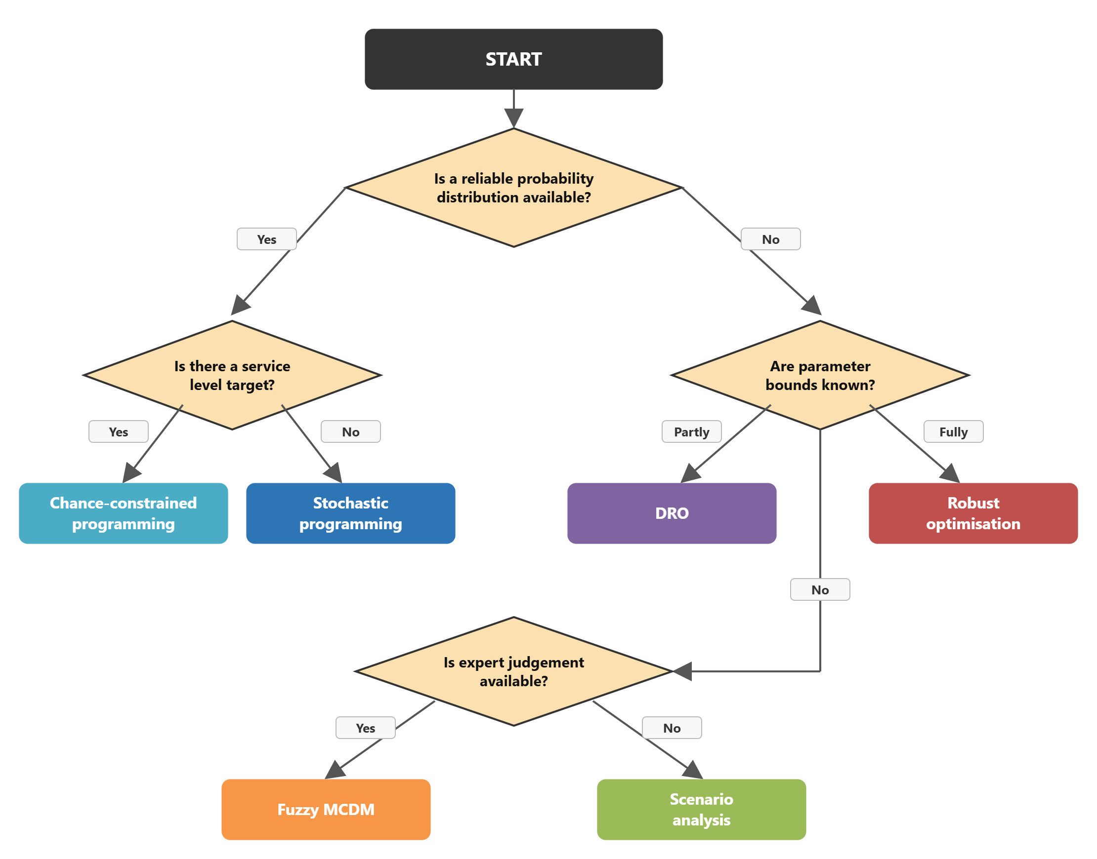
Figure 5. Decision flowchart for selecting an approach.
6. Challenges and Future Directions
6.1 Current Challenges
Wider use of OUU in health care faces several obstacles. First, data quality and availability: stochastic models need reliable probability distributions, yet many health organisations lack the data infrastructure for this level of analysis. Second, computational complexity: solution time grows exponentially as the dimensions of uncertainty increase. Third, the implementation gap: many sophisticated models developed in the academic literature cannot be applied in real hospital settings. Fourth, multi-stakeholder decision making: hospital decisions emerge from interaction among clinicians, managers, nurses and policy makers rather than from a single manager. Fifth, explainability: acceptance of AI-supported models in clinical settings depends on results being explained transparently to decision makers.
6.2 Future Directions
Integration of machine learning and optimisation is becoming widespread. Shehadeh and Padman (2023) combined machine-learning prediction of surgery duration with optimisation models to exploit the strengths of both. Ning and You (2019) expected deep-learning-based demand forecasting, adaptive policies from reinforcement learning and scenario generation with generative adversarial networks to shape the future of OUU. Real-time data use is another major trend: the internet of things and electronic health records allow models to be updated continuously. Health-management-specific adaptations of moment-based and Wasserstein-based DRO formulations are a promising research area. Pandemic preparedness also remains topical: COVID-19 showed that the resilience of health systems to sudden demand surges must be strengthened with optimisation models.
Recommendation for Türkiye: hospital information systems and e-Nabız already hold the arrival, length-of-stay, surgery-duration and stock data that these models need. A practical first step is for hospital quality and operations units to estimate empirical distributions for a few high-impact decisions (operating room blocks, blood and vaccine stock, ICU beds) and to report EMV and CVaR side by side, so that patient-safety tail risks are visible in routine management decisions.
7. Synthesis and Conclusion
Optimisation under uncertainty is an indispensable tool for improving decision quality in health management. The seven core approaches covered here (scenario analysis, stochastic programming, robust optimisation, DRO, chance-constrained programming, fuzzy multi-criteria decision making and simulation-based optimisation) respond to different levels of uncertainty and decision contexts.
The key lessons are as follows. First, correctly diagnosing the type of uncertainty is a precondition for choosing the right method: aleatory uncertainty calls for stochastic tools, epistemic uncertainty for robust or fuzzy tools. Second, there is no single “best method”; every approach has strengths and limitations. Third, expected value alone is not enough in health management; tail-risk measures such as CVaR are essential for protecting patient safety in critical areas such as blood banks and emergency drug stocks. Fourth, PubMed evidence shows that these methods deliver concrete, measurable improvements, such as a 44.55% shorter length of stay, 9.8% fewer ICU beds and 37% shorter preparation time. Fifth, every model’s assumptions should be stated explicitly and their limits of validity presented transparently to decision makers.
Looking ahead, combining AI-supported forecasting with OUU is especially promising. The health systems of the future will treat uncertainty not as an enemy but as a reality to be managed systematically, with decision support systems built accordingly. Even so, the clinical applicability of these hybrid approaches is still limited, and explainability and computational complexity remain the main barriers. The nine worked problems in this chapter aim to show the concrete health care counterparts of theoretical concepts; when applying the models in the real world, the simplifying assumptions made here must be assessed carefully and relaxed where necessary.
Appendix: Notation and Abbreviations
| Symbol or abbreviation | Meaning | Health management interpretation |
|---|---|---|
| x | First-stage decision variable | Decision taken before uncertainty is revealed (beds, order quantity) |
| y | Second-stage (recourse) variable | Corrective action afterwards (overtime, emergency order) |
| ξ | Uncertain parameter vector | Demand, durations, arrivals |
| f(x, ξ), g(x, ξ) | Objective and constraint functions | Cost, profit or time; capacity or waiting-time conditions |
| Q(x, ξ) | Recourse function | Second-stage correction cost |
| X, U, 𝒫 | Feasible set, uncertainty set, ambiguity set of distributions | Allowed decisions; range of parameters (RO); possible distributions (DRO) |
| α | Accepted violation probability | Confidence level 1 − α in chance constraints |
| μ, σ, σ² | Mean, standard deviation, variance | Average demand or duration and its variability |
| Φ, φ | Standard normal CDF and PDF | Used in chance constraints and loss functions |
| pₛ | Probability of scenario s | Weight of a demand scenario |
| EMV / EV | Expected monetary value / expected value | Probability-weighted average cost or profit |
| EVPI, EVwPI | Expected value of perfect information; expected value with perfect information | Value of a perfect forecast: EMV* − EVwPI |
| VaR, CVaR | Value at Risk; Conditional Value at Risk | Worst loss at a confidence level; average loss beyond it |
| CR | Critical ratio Cᵤ / (Cᵤ + Cₒ) | Newsvendor threshold for blood, vaccine and drug stock |
| SP, RO, DRO, CCP | Stochastic programming, robust optimisation, distributionally robust optimisation, chance-constrained programming | The core OUU families |
| MILP, MINLP | Mixed-integer (non)linear programming | Models with integer decisions such as beds or staff |
| FMCDM | Fuzzy multi-criteria decision making | Expert-judgement-based selection |
How to cite
This article is the English version of the technical report: Kurutkan, M. N. (2026). Belirsizlik altında optimizasyon: Operasyon yönetiminden sağlık yönetimine; kavramlar, yaklaşımlar, kanıtlar ve çözümlü problemler [Optimisation under uncertainty, from operations to health management: Concepts, approaches, evidence and worked problems] (Technical report). Düzce University, Faculty of Business, Department of Health Management. https://www.researchgate.net/publication/403611582
References
Arab Momeni, M., Mostofi, A., Jain, V., & Soni, G. (2022). COVID19 epidemic outbreak: Operating rooms scheduling, specialty teams timetabling and emergency patients’ assignment using the robust optimization approach. Annals of Operations Research, 1–31. https://doi.org/10.1007/s10479-022-04667-7
Aslani, N., Kuzgunkaya, O., Vidyarthi, N., & Terekhov, D. (2021). A robust optimization model for tactical capacity planning in an outpatient setting. Health Care Management Science, 24(1), 26–40. https://doi.org/10.1007/s10729-020-09528-y
Balasubramanian, J., & Grossmann, I. E. (2003). Scheduling optimization under uncertainty: An alternative approach. Computers and Chemical Engineering, 27(4), 469–490.
Ben-Tal, A., El Ghaoui, L., & Nemirovski, A. (2009). Robust optimization. Princeton University Press.
Bertsimas, D., & Sim, M. (2004). The price of robustness. Operations Research, 52(1), 35–53.
Birge, J. R., & Louveaux, F. (2011). Introduction to stochastic programming (2nd ed.). Springer.
Büyüközkan, G., Çifçi, G., & Güleryüz, S. (2011). Strategic analysis of healthcare service quality using fuzzy AHP methodology. Expert Systems with Applications, 38(8), 9407–9424.
Daldoul, D., Nouaouri, I., Bouchriba, H., & Allaoui, H. (2023). Impact of an approach combining optimization and simulation to improve the service quality of an emergency department. La Tunisie Médicale, 101(4), 404–409.
Denton, B., Viapiano, J., & Vogl, A. (2010). Optimization of surgery sequencing and scheduling decisions under uncertainty. Health Care Management Science, 10(1), 13–24.
Diwekar, U. M., & Kalagnanam, J. R. (1997). Efficient sampling technique for optimization under uncertainty. AIChE Journal, 43(2), 440–447.
Engau, A., & Sigler, D. (2020). Pareto solutions in multicriteria optimization under uncertainty. European Journal of Operational Research, 281(2), 357–368.
Fariman, S. K., Danesh, K., Pourtalebiyan, M., Fakhri, Z., Motallebi, A., & Fozooni, A. (2024). A robust optimization model for multi-objective blood supply chain network considering scenario analysis under uncertainty. Scientific Reports, 14(1), 9452. https://doi.org/10.1038/s41598-024-57521-0
Guth, P. A., & Van Barel, A. (2023). Multilevel quasi-Monte Carlo for optimization under uncertainty. Numerische Mathematik, 154(3–4), 443–484.
Halawa, F., Madathil, S. C., Gittler, A., & Khasawneh, M. T. (2020). Advancing evidence-based healthcare facility design: A systematic literature review. Health Care Management Science, 23(3), 453–480. https://doi.org/10.1007/s10729-020-09506-4
Heizer, J., Render, B., & Munson, C. (2020). Operations management: Sustainability and supply chain management (13th ed.). Pearson.
Hill, P., Lederman, J., Jonsson, D., Bolin, P., & Vicente, V. (2025). Understanding EMS response times: A machine learning-based analysis. BMC Medical Informatics and Decision Making, 25(1), 143. https://doi.org/10.1186/s12911-025-02975-z
Hoffmans-Holtzer, N., Smolenaers, L., Olofsen-van Acht, M., Hoogeman, M., Balvert, M., & Petit, S. (2024). Robust optimization of a radiotherapy pretreatment preparation workflow. Physics in Medicine and Biology, 69(2). https://doi.org/10.1088/1361-6560/acf437
Jensen, F. V., & Nielsen, T. D. (2011). Probabilistic decision graphs for optimization under uncertainty. 4OR, 9(1), 1–28.
Jensen, F. V., & Nielsen, T. D. (2013). Probabilistic decision graphs for optimization under uncertainty. Annals of Operations Research, 204(1), 223–248.
Jiang, R., & Guan, Y. (2016). Data-driven chance constrained stochastic program. Mathematical Programming, 158(1–2), 291–327.
Jin, R., Du, X., & Chen, W. (2003). The use of metamodeling techniques for optimization under uncertainty. Structural and Multidisciplinary Optimization, 25(2), 99–116.
Köbis, E., & Tammer, C. (2023). Optimality conditions in optimization under uncertainty. Journal of Nonlinear and Variational Analysis, 7(5), 769–784.
Liu, Y., & Gunawan, R. (2017). Bioprocess optimization under uncertainty using ensemble modeling. Journal of Biotechnology, 244, 34–44.
Masic, I. (2022). Medical decision making: An overview. Acta Informatica Medica, 30(3), 230–235. https://doi.org/10.5455/aim.2022.30.230-235
Mishra, A. A., Mukhopadhaya, J., Alonso, J., & Iaccarino, G. (2020). Design exploration and optimization under uncertainty. Physics of Fluids, 32(8), 085106.
Ng, L. W. T., & Willcox, K. E. (2014). Multifidelity approaches for optimization under uncertainty. International Journal for Numerical Methods in Engineering, 100(10), 746–772.
Ning, C., & You, F. (2019). Optimization under uncertainty in the era of big data and deep learning. Computers and Chemical Engineering, 125, 434–448.
Papamichail, I., et al. (2025). Optimizing patient flow logistics: Strategic challenges, tactical solutions, and future directions. BMC Health Services Research. https://doi.org/10.1186/s12913-025-13516-9
Rockafellar, R. T., & Wets, R. J.-B. (1991). Scenarios and policy aggregation in optimization under uncertainty. Mathematics of Operations Research, 16(1), 119–147.
Roshanaei, V., Luong, C., Aleman, D. M., & Urbach, D. R. (2017). Collaborative operating room planning and scheduling. INFORMS Journal on Computing, 29(3), 558–580.
Saghafian, S., Hopp, W. J., Van Oyen, M. P., Desmond, J. S., & Kronick, S. L. (2015). Patient streaming as a mechanism for improving responsiveness in emergency departments. Operations Research, 63(5), 1011–1029.
Shapiro, A., Dentcheva, D., & Ruszczyński, A. (2021). Lectures on stochastic programming (3rd ed.). SIAM.
Shehadeh, K. S., & Padman, R. (2022). Quantile regression forests for individualized surgery scheduling. Health Care Management Science, 25(4). https://doi.org/10.1007/s10729-022-09609-0
Shehadeh, K. S., & Padman, R. (2023). Surgical scheduling via optimization and machine learning with long-tailed data. Health Care Management Science. https://doi.org/10.1007/s10729-023-09649-0
Tolpin, D., & Shimony, S. E. (2012). Semimyopic measurement selection for optimization under uncertainty. IEEE Transactions on Systems, Man, and Cybernetics, Part B, 42(2), 565–579.
Vassiliadis, C. G., & Pistikopoulos, E. N. (2001). Maintenance scheduling and process optimization under uncertainty. Computers and Chemical Engineering, 25(2–3), 217–236.
Wan, F., Fondrevelle, J., Wang, T., & Duclos, A. (2023). Two-stage multi-objective optimization for ICU bed allocation under multiple sources of uncertainty. Scientific Reports, 13(1), 18925. https://doi.org/10.1038/s41598-023-45777-x
Wendt, M., Li, P., & Wozny, G. (2002). Nonlinear chance-constrained process optimization under uncertainty. Industrial and Engineering Chemistry Research, 41(15), 3621–3629.
Yeung, W. S. T., et al. (2016). Stochastic multi-objective auto-optimization for resource allocation decision-making in fixed-input health systems. Health Care Management Science, 19(4). https://doi.org/10.1007/s10729-015-9350-2
Key concepts in this article
Waiting time Discrete-event simulation Length of stay Patient flow Forecasting Monte Carlo simulation Machine learning Pandemic preparedness Cost-effectiveness analysis Electronic health record (EHR) Reliability Systematic review Artificial intelligence (AI)Concepts link to the Glossary. Explore the knowledge graph →
Cite this page (APA 7)
Kurutkan, M. N. (2026, November 11). Optimisation Under Uncertainty, from Operations to Health Management: Concepts, Approaches, Evidence and Worked Problems. The Health Topics. https://healthtopic.org/topics/optimisation-under-uncertainty-from-operations-to-health-management-concepts-approaches-evidence-and-worked-problems/